Diagnostics for approximate likelihood ratios

Kyle Cranmer, Juan Pavez, Gilles Louppe, March 2016.

This is an extension of the example in Parameterized inference from multidimensional data. To aid in visualization, we restrict to a 1-dimensional slice of the likelihood along $\alpha$ with $\beta=-1$. We consider three situations: i) a poorly trained, but well calibrated classifier; ii) a well trained, but poorly calibrated classifier; and iii) a well trained, and well calibrated classifier. For each case, we employ two diagnostic tests. The first checks for independence of $-2\log\Lambda(\theta)$ with respect to changes in the reference value $\theta_1$. The second uses a classifier to distinguish between samples from $p(\mathbf{x}|\theta_0)$ and samples from $p(\mathbf{x}|\theta_1)$ weighted according to $r(\mathbf{x}; \theta_0, \theta_1)$.

%matplotlib inline
import matplotlib.pyplot as plt

import numpy as np
import theano
from scipy.stats import chi2
from itertools import product

np.random.seed(314)

Create model and generate artificial data

from carl.distributions import Join
from carl.distributions import Mixture
from carl.distributions import Normal
from carl.distributions import Exponential
from carl.distributions import LinearTransform
from sklearn.datasets import make_sparse_spd_matrix

# Parameters
true_A = 1.
A = theano.shared(true_A, name="A")

# Build simulator
R = make_sparse_spd_matrix(5, alpha=0.5, random_state=7)

p0 = LinearTransform(Join(components=[
        Normal(mu=A, sigma=1),
        Normal(mu=-1, sigma=3),
        Mixture(components=[Normal(mu=-2, sigma=1),
                            Normal(mu=2, sigma=0.5)]),
        Exponential(inverse_scale=3.0),
        Exponential(inverse_scale=0.5)]), R)

# Define p1 at fixed arbitrary value A=0
p1s = []
p1_params = [(0,-1),(1,-1),(0,1)]
for p1_p in p1_params:
    p1s.append(LinearTransform(Join(components=[
        Normal(mu=p1_p[0], sigma=1),
        Normal(mu=p1_p[1], sigma=3),
        Mixture(components=[Normal(mu=-2, sigma=1),
                            Normal(mu=2, sigma=0.5)]),
        Exponential(inverse_scale=3.0),
        Exponential(inverse_scale=0.5)]), R))
p1 = p1s[0]

# Draw data
X_true = p0.rvs(500, random_state=314)

Known likelihood setup

# Minimize the exact LR
from scipy.optimize import minimize

p1 = p1s[2]

def nll_exact(theta, X):
    A.set_value(theta[0])
    return (p0.nll(X) - p1.nll(X)).sum()

r = minimize(nll_exact, x0=[0], args=(X_true,))
exact_MLE = r.x

print("Exact MLE =", exact_MLE)

('Exact MLE =', array([ 1.01185166]))

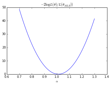
# Exact LR
A.set_value(true_A)
nlls = []
As_ = []
bounds = [(true_A - 0.30, true_A + 0.30)]
As = np.linspace(bounds[0][0],bounds[0][1], 100)
nll = [nll_exact([a], X_true) for a in As]
nll = np.array(nll)
nll = 2. * (nll - r.fun)

plt.plot(As, nll)
plt.xlabel(r"$\alpha$")
plt.title(r"$-2 \log L(\theta) / L(\theta_{MLE}))$")
plt.show()

png

Likelihood-free setup

Here we create the data to train a parametrized classifier

# Build classification data
from carl.learning import make_parameterized_classification

bounds = [(-3, 3), (-3, 3)]

clf_parameters = [(1000, 100000), (1000000, 500), (1000000, 100000)]
X = [0]*3*3
y = [0]*3*3

for k,(param,p1) in enumerate(product(clf_parameters,p1s)):
    X[k], y[k] = make_parameterized_classification(
        p0, p1,
        param[0], 
        [(A, np.linspace(bounds[0][0],bounds[0][1], num=30))],
        random_state=0)

# Train parameterized classifier
from carl.learning import as_classifier
from carl.learning import make_parameterized_classification
from carl.learning import ParameterizedClassifier
from sklearn.neural_network import MLPRegressor
from sklearn.pipeline import make_pipeline
from sklearn.preprocessing import StandardScaler

clfs = []

for k, _ in enumerate(product(clf_parameters,p1s)):
    clfs.append(ParameterizedClassifier(
        make_pipeline(StandardScaler(), 
                  as_classifier(MLPRegressor(learning_rate="adaptive", 
                                             hidden_layer_sizes=(40, 40),
                                             tol=1e-6,
                                             random_state=0))),
        [A]))
    clfs[k].fit(X[k], y[k])

from carl.learning import CalibratedClassifierCV
from carl.ratios import ClassifierRatio

def vectorize(func,n_samples,clf,p1):
    def wrapper(X):
        v = np.zeros(len(X))

        for i, x_i in enumerate(X):
            v[i] = func(x_i,n_samples=n_samples,clf=clf, p1=p1)

        return v.reshape(-1, 1)

    return wrapper

def objective(theta, random_state=0, n_samples=100000, clf=clfs[0],p1=p1s[0]):    
    # Set parameter values   
    A.set_value(theta[0])

    # Fit ratio
    ratio = ClassifierRatio(CalibratedClassifierCV(
        base_estimator=clf, 
        cv="prefit",  # keep the pre-trained classifier
        method="histogram", bins=50))

    X0 = p0.rvs(n_samples=n_samples)
    X1 = p1.rvs(n_samples=n_samples, random_state=random_state)
    X = np.vstack((X0, X1))
    y = np.zeros(len(X))
    y[len(X0):] = 1

    ratio.fit(X, y)

    # Evaluate log-likelihood ratio
    r = ratio.predict(X_true, log=True)
    value = -np.mean(r[np.isfinite(r)])  # optimization is more stable using mean
                                         # this will need to be rescaled by len(X_true)    

    return value

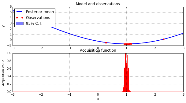
Now we use a Bayesian optimization procedure to create a smooth surrogate of the approximate likelihood.

from GPyOpt.methods import BayesianOptimization

solvers = []

for k, (param, p1) in enumerate(product(clf_parameters,p1s)):
    clf = clfs[k]
    n_samples = param[1]
    bounds = [(-3, 3)]
    solvers.append(BayesianOptimization(vectorize(objective,n_samples,clf,p1), bounds))
    solvers[k].run_optimization(max_iter=50, true_gradients=False)

approx_MLEs = []

for k, _ in enumerate(product(clf_parameters,p1s)):
    solver = solvers[k]
    approx_MLE = solver.x_opt
    approx_MLEs.append(approx_MLE)
    print("Approx. MLE =", approx_MLE)

('Approx. MLE =', array([ 1.1567223]))
('Approx. MLE =', array([ 1.12968218]))
('Approx. MLE =', array([ 1.27133084]))
('Approx. MLE =', array([ 1.09549403]))
('Approx. MLE =', array([ 0.91981054]))
('Approx. MLE =', array([ 0.77314181]))
('Approx. MLE =', array([ 1.02540673]))
('Approx. MLE =', array([ 1.00016057]))
('Approx. MLE =', array([ 1.0148428]))

solver.plot_acquisition()

png

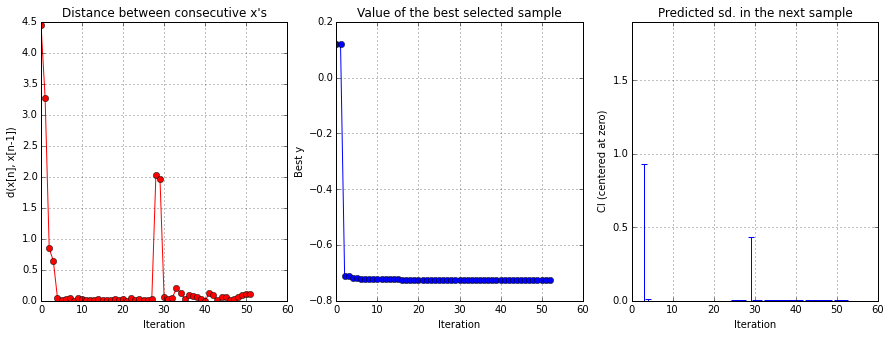
solver.plot_convergence()

png

# Minimize the surrogate GP approximate of the approximate LR
rs = []
solver = solvers[0]

for k, _ in enumerate(product(clf_parameters,p1s)):
    def gp_objective(theta):
        theta = theta.reshape(1, -1)
        return solvers[k].model.predict(theta)[0][0]

    r = minimize(gp_objective, x0=[0])
    rs.append(r)
    gp_MLE = r.x

    print("GP MLE =", gp_MLE)

('GP MLE =', array([ 1.15409679]))
('GP MLE =', array([ 1.13815972]))
('GP MLE =', array([ 1.25892465]))
('GP MLE =', array([ 1.03389187]))
('GP MLE =', array([ 0.93057811]))
('GP MLE =', array([ 0.7587189]))
('GP MLE =', array([ 1.01290299]))
('GP MLE =', array([ 1.00689144]))
('GP MLE =', array([ 0.99879448]))

#bounds = [(exact_MLE[0] - 0.16, exact_MLE[0] + 0.16)]

approx_ratios = []
gp_ratios = []
gp_std = []
gp_q1 = []
gp_q2 = []
n_points = 30

for k,(param,p1) in enumerate(product(clf_parameters,p1s)):
    clf = clfs[k]
    n_samples = param[1]
    solver = solvers[k]
    #As = np.linspace(*bounds[0], 100)
    nll_gp, var_gp = solvers[k].model.predict(As.reshape(-1, 1))
    nll_gp = 2. * (nll_gp - rs[k].fun) * len(X_true)
    gp_ratios.append(nll_gp)

    # STD
    std_gp = np.sqrt(4*var_gp*len(X_true)*len(X_true))
    std_gp[np.isnan(std_gp)] = 0.
    gp_std.append(std_gp)

    # 95% CI
    q1_gp, q2_gp = solvers[k].model.predict_quantiles(As.reshape(-1, 1))
    q1_gp = 2. * (q1_gp - rs[k].fun) * len(X_true)
    q2_gp = 2. * (q2_gp - rs[k].fun) * len(X_true)
    gp_q1.append(q1_gp)
    gp_q2.append(q2_gp)

Plots for the first diagonstic: $\theta_1$-independence

bounds = [(true_A - 0.30, true_A + 0.30)]

for k, _ in enumerate(clf_parameters):
    fig = plt.figure()
    ax = fig.add_subplot(1,1,1)
    ax.plot(As, nll, label="Exact")
    #plt.plot(np.linspace(*bounds[0], n_points), nll_approx - , label="approx.")
    #plt.plot(np.linspace(bounds[0][0],bounds[0][1], n_points), nll_approx , label="approx.")
    ax.plot(As, gp_ratios[3*k], label=r"Approx., $\theta_1=(\alpha=0,\beta=-1)$")
    ax.plot(As, gp_ratios[3*k+1], label=r"Approx., $\theta_1=(\alpha=1,\beta=-1)$")
    ax.fill_between(As,(gp_ratios[3*k] - gp_std[3*k]).ravel(),(gp_ratios[3*k] + gp_std[3*k]).ravel(),
                     color='g',alpha=0.2)
    ax.plot(As, gp_ratios[3*k+2], label=r"Approx., $\theta_1=(\alpha=0,\beta=1)$")
    handles, labels = ax.get_legend_handles_labels()
    ax.set_xlabel(r"$\alpha$")
    ax.set_ylabel(r"$-2 \log \Lambda(\theta)$")
    #plt.legend()
    p5 = plt.Rectangle((0, 0), 0.2, 0.2, fc="green",alpha=0.2,edgecolor='none')
    handles.insert(4,p5)
    labels.insert(4,r"$\pm 1 \sigma$, $\theta_1=(\alpha=0,\beta=-1)$")
    handles[1],handles[-2] = handles[-2],handles[1]
    labels[1],labels[-2] = labels[-2],labels[1]

    ax.legend(handles,labels)
    ax.set_ylim(0, 14)
    ax.set_xlim(bounds[0][0],bounds[0][1])
    plt.savefig('likelihood_comp_{0}.pdf'.format(k))
    plt.show()

png

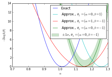
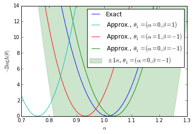
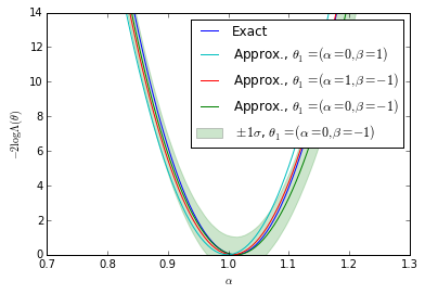
We show the posterior mean of a Gaussian processes resulting from Bayesian optimization of the raw approximate likelihood. In addition, the standard deviation of the Gaussian process is shown for one of the $\theta_1$ reference points to indicate the size of these statistical fluctuations. It is clear that in the well calibrated cases that these fluctuations are small, while in the poorly calibrated case these fluctuations are large. Moreover, in the first case we see that in the poorly trained, well calibrated case the classifier $\hat{s}(\mathbf{x}; \theta_0, \theta_1)$ has a significant dependence on the $\theta_1$ reference point. In contrast, in the second case the likelihood curves vary significantly, but this is comparable to the fluctuations expected from the calibration procedure. Finally, the third case shows that in the well trained, well calibrated case that the likelihood curves are all consistent with the exact likelihood within the estimated uncertainty band of the Gaussian process.

The second diagnostic - ROC curves for a discriminator

from sklearn.metrics import roc_curve, auc

def makeROC(predictions ,targetdata):
    fpr, tpr, _  = roc_curve(targetdata.ravel(),predictions.ravel())
    roc_auc = auc(fpr, tpr)

    return fpr,tpr,roc_auc

# I obtain data from r*p1 by resampling data from p1 using r as weights
def weight_data(x0,x1,weights):
    x1_len = x1.shape[0]
    weights = weights / weights.sum()
    weighted_data = np.random.choice(range(x1_len), x1_len, p = weights)
    w_x1 = x1.copy()[weighted_data]
    y = np.zeros(x1_len * 2)
    x_all = np.vstack((w_x1,x0))
    y_all = np.zeros(x1_len * 2)
    y_all[x1_len:] = 1
    return (x_all,y_all)

p1 = p1s[0]
X0_roc = p0.rvs(500000,random_state=777)
X1_roc = p1.rvs(500000,random_state=777)

# Roc curve comparison for p0 - r*p1
for k,param in enumerate(clf_parameters):
    #fig.add_subplot(3,2,(k+1)*2)

    clf = clfs[3*k]
    n_samples = param[1]
    X0 = p0.rvs(n_samples)
    X1 = p1.rvs(n_samples,random_state=777)
    X_len = X1.shape[0]
    ratio = ClassifierRatio(CalibratedClassifierCV(
        base_estimator=clf, 
        cv="prefit",  # keep the pre-trained classifier
        method="histogram", bins=50))

    X = np.vstack((X0, X1))
    y = np.zeros(len(X))
    y[len(X0):] = 1

    ratio.fit(X, y)

    # Weighted with true ratios
    true_r = p0.pdf(X1_roc) / p1.pdf(X1_roc)
    true_r[np.isinf(true_r)] = 0.
    true_weighted = weight_data(X0_roc,X1_roc,true_r)
    # Weighted with approximated ratios
    app_r = ratio.predict(X1_roc,log=False)
    app_r[np.isinf(app_r)] = 0.
    app_weighted = weight_data(X0_roc,X1_roc,app_r)

    clf_true = MLPRegressor(tol=1e-05, activation="logistic", 
                   hidden_layer_sizes=(10, 10), learning_rate_init=1e-07, 
                   learning_rate="constant", algorithm="l-bfgs", random_state=1, 
                   max_iter=75)
    clf_true.fit(true_weighted[0],true_weighted[1])
    predicted_true = clf_true.predict(true_weighted[0])
    fpr_t,tpr_t,roc_auc_t = makeROC(predicted_true, true_weighted[1])
    plt.plot(fpr_t, tpr_t, label=r"$p(x|\theta_1)r(x|\theta_0,\theta_1)$ exact" % roc_auc_t)

    clf_true.fit(np.vstack((X0_roc,X1_roc)),true_weighted[1])
    predicted_true = clf_true.predict(np.vstack((X0_roc,X1_roc)))
    fpr_f,tpr_f,roc_auc_f = makeROC(predicted_true, true_weighted[1])
    plt.plot(fpr_f, tpr_f, label=r"$p(x|\theta_1)$ no weights" % roc_auc_f)

    clf_true.fit(app_weighted[0],app_weighted[1])
    predicted_true = clf_true.predict(app_weighted[0])
    fpr_a,tpr_a,roc_auc_a = makeROC(predicted_true, app_weighted[1])
    plt.plot(fpr_a, tpr_a, label=r"$p(x|\theta_1)r(x|\theta_0,\theta_1)$ approx." % roc_auc_a)

    plt.plot([0, 1], [0, 1], 'k--')
    plt.xlim([0.0, 1.0])
    plt.ylim([0.0, 1.05])
    plt.xlabel('False Positive Rate')
    plt.ylabel('True Positive Rate')
    plt.legend(loc="lower right")
    plt.tight_layout()

    plt.savefig('ROC_comp{0}.pdf'.format(k))
    plt.show()

#plt.tight_layout()
#plt.savefig('all_comp.pdf'.format(k))

png

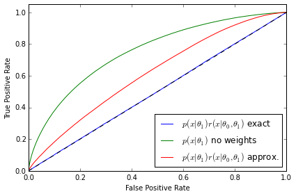
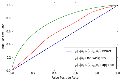
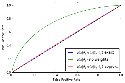
The ROC curves tell a similarly revealing story. As expected, the classifier is not able to distinguish between the distributions when $p(\mathbf{x}|\theta_1)$ is weighted by the exact likelihood ratio. We can also rule out that this is a deficiency in the classifier because the two distributions are well separated when no weights are applied to $p(\mathbf{x}|\theta_1)$. In both the first and second examples the ROC curve correctly diagnoses deficiencies in the approximate likelihood ratio $\hat{r}(\hat{s}(\mathbf{x}; \theta_0, \theta_1))$. Finally, third example shows that the ROC curve in the well trained, well calibrated case is almost identical with the exact likelihood ratio, confirming the quality of the approximation.

Index